Decision Tree
A Decision Tree is a supervised machine learning algorithm used for both classification and regression tasks. It models decisions based on a tree-like structure where each internal node represents a feature (attribute), each branch represents a decision rule, and each leaf node represents an outcome (class label or regression value).
- Root Node: : The top node that represents the entire dataset, which is split into two or more homogeneous sets.
- Internal Nodes: Represent tests on features, leading to further splits.
- Leaf Nodes: Terminal nodes that represent the final output (class label in classification or a continuous value in regression).
How It Works
The algorithm involves the following steps:
- Splitting: Divides nodes into subsets based on features and thresholds. Metrics like Gini Impurity or Information Gain are used.
- Decision Rules: Each internal node corresponds to a feature and a threshold value that decides how to split the data. For example, if a feature is "Age" and the threshold is 30, the split will separate instances where "Age <= 30" from those where "Age > 30".
- Stopping Criteria: Stops splitting based on conditions like maximum depth or minimum samples in a node.
- Pruning: After building the tree, pruning may be performed to reduce overfitting. This involves removing nodes that have little importance, which simplifies the model and enhances its generalization to unseen data.
Code
# Import libraries
from sklearn.tree import DecisionTreeClassifier
from sklearn.datasets import load_iris
from sklearn.model_selection import train_test_split
from sklearn.metrics import accuracy_score

# Load dataset
dataset = load_iris()
X, y = dataset.data, dataset.target

# Train-test split
X_train, X_test, y_train, y_test = train_test_split(X, y, test_size=0.3)

# Create and train the model
classifier = DecisionTreeClassifier()
classifier.fit(X_train, y_train)

# Make predictions
y_predict = classifier.predict(X_test)

# Evaluate accuracy
print("Accuracy:", accuracy_score(y_test, y_predict))

# Visualize the tree
from sklearn import tree
tree.plot_tree(classifier)
Accuracy: 0.93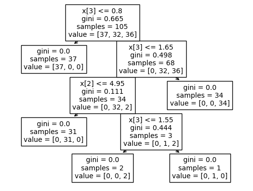 Decision Tree Visualization
# Scatter plot for actual vs predicted values
import matplotlib.pyplot as plt
plt.scatter(y_test, y_predict, alpha=0.7, color='blue')
plt.title('Actual vs Predicted Values')
plt.xlabel('Actual Values')
plt.ylabel('Predicted Values')
plt.grid(True)
plt.axis('equal')
plt.show()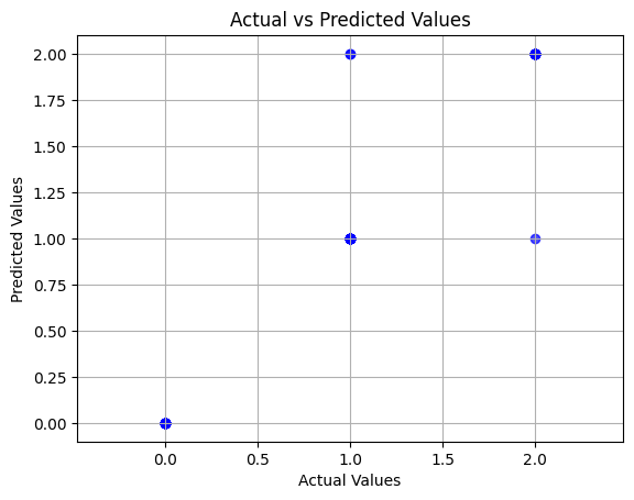 Scatter Plot: Actual vs Predicted Values
Advantages and Disadvantages
| Advantages | Disadvantages |
|---|---|
| Interpretability: Easy to understand and visualize. | Overfitting: Can become complex and overfit if not pruned. |
| Non-linear Relationships: Models non-linear relationships effectively. | Instability: Small changes in data can result in different splits. |
| Feature Importance: Provides insights into the importance of features. | Bias: May favor features with more levels, leading to suboptimal splits. |
Applications
- Finance: Credit scoring, risk assessment.
- Healthcare: Diagnosing diseases based on patient data.
- Marketing: Customer segmentation and targeting.