Support Vector Machines (SVM)

Support Vector Machines (SVM) are supervised machine learning models used for classification and regression tasks. SVM is popular for classification problems and works by finding the hyperplane that best separates different classes of data. The hyperplane is chosen to maximize the margin between the two classes.

Key Concepts

• Support Vectors: Data points closest to the hyperplane. These influence the hyperplane's position and orientation.
• Margin: The distance between the hyperplane and the support vectors. SVM maximizes this margin.
• Kernel Trick: Enables SVM to handle non-linear boundaries by transforming data into a higher-dimensional space using functions like RBF or Polynomial kernels.

Mathematical Intuition

The objective of SVM is to find a hyperplane in an \( N \)-dimensional space (where \( N \) is the number of features) that distinctly classifies the data points. The equation for the hyperplane is:

• \( w \): Weight vector
• \( x \): Feature vector
• \( b \): Bias term

For a point on the margin:

• \( w^T x + b = 1 \) for the positive class
• \( w^T x + b = -1 \) for the negative class

The margin is computed as the perpendicular distance between these margins and the hyperplane. SVM maximizes this margin for better generalization.

Implementation

from sklearn.datasets import make_classification
from sklearn.model_selection import train_test_split
from sklearn.svm import SVC
from sklearn.metrics import accuracy_score, classification_report

# Generate synthetic data
X, y = make_classification(random_state=42, n_samples=1000, n_features=2, n_informative=2, n_redundant=0)

# Train-test split
X_train, X_test, y_train, y_test = train_test_split(X, y, test_size=0.2, random_state=42)

# Train the SVM model
model = SVC(kernel='linear')
model.fit(X_train, y_train)

# Test the model
y_pred = model.predict(X_test)
accuracy = accuracy_score(y_test, y_pred)
print("Accuracy:", accuracy)

# Classification report
print(classification_report(y_test, y_pred))

Accuracy: 0.88
Classification Report:
              precision    recall  f1-score   support
           0       0.88      0.88      0.88       101
           1       0.88      0.88      0.88        99

    accuracy                           0.88       200
   macro avg       0.88      0.88      0.88       200
weighted avg       0.88      0.88      0.88       200

Hyperparameter Tuning

• C: Regularization parameter controlling the trade-off between maximizing the margin and correctly classifying training points. Smaller \( C \) widens the margin but allows more misclassifications.
• Kernel: Determines the decision boundary shape. Common kernels include:
  • linear: Linear hyperplane
  • poly: Polynomial kernel
  • rbf: Radial Basis Function (Gaussian)

Visualization

Visualization using two features:

import numpy as np
import matplotlib.pyplot as plt

# Select First 2 features as X and Y
X_vis = X[:, :2] 

# Find min and max of both columns
x_min, x_max = X[:, 0].min() - 1, X[:, 0].max() + 1
y_min, y_max = X[:, 1].min() - 1, X[:, 1].max() + 1

# Construct a meshgrid - a list of coordinates
h = 0.01 # Step
x_coordinates, y_coordinates = np.arange(x_min, x_max, h), np.arange(y_min, y_max, h)
xx, yy = np.meshgrid(x_coordinates, y_coordinates)

# Decision boundary
x_1d, y_1d = xx.ravel(), yy.ravel() # Convert 2D to 1D
values_1d = np.c_[x_1d, y_1d] # Concatenate
Z = model.decision_function(values_1d)
Z = Z.reshape(xx.shape)

plt.scatter(X_vis[:, 0], X_vis[:, 1], c=y, cmap='viridis', alpha=0.7)
plt.contourf(xx, yy, Z, levels=[-1, 0, 1], colors='c', alpha=0.5)
plt.contour(xx, yy, Z, levels=[-1, 0, 1], colors='r', alpha=0.5, linestyles=['--', '-', '--'])
plt.xlabel('Feature 1')
plt.ylabel('Feature 2')
plt.title('SVM Decision Boundary')
plt.show()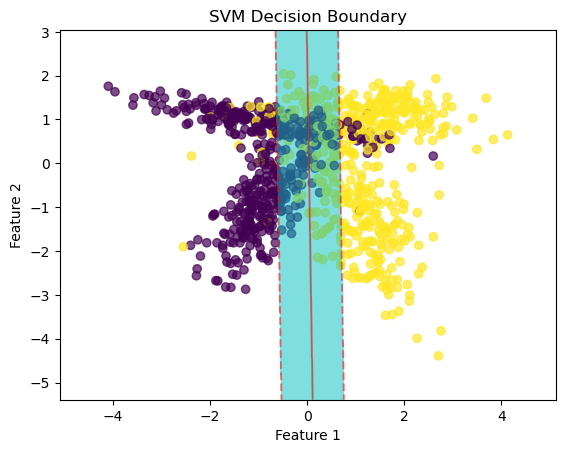

SVM Decision Boundary

Soft Margin Formulation

Soft margin SVM allows certain misclassifications to ensure a wider margin, helping the model generalize better to unseen data. The \( C \) parameter controls the trade-off between margin width and misclassification.

Errors in SVM

• Classification Error: When a data point is misclassified.
• Margin Error: When a data point falls within the margin.